Goals

In this tutorial, we will:

• Review creating scatterplots using geom_point
• Add a best fit line to your scatterplot
• Create a simple linear model using the lm function.
• Predict response values from an inputted predictor value

What is Linear Regression?

Linear Regression (or you may also call it "Linear Modeling") is the statistical process of fitting and predicting responses to a numeric variable using one or more predictor variables in the form of a linear equation.

"Simple Linear" Model

If we are only using one predictor variable, then we can call it a "Simple" model.

If the response variable is numeric, and we are using the equation of a line to model its relationship with one predictor, then it is called a "Simple Linear" Model.

Introduce some Data

The palmerpenguins package contains a built in dataset named penguins that has information on 344 penguins body measurements.

library(palmerpenguins)
penguins

A Guiding question

One question we might have is: How we might model (predict) a penguin's flipper length by other penguin features?"

Let's focus on using body mass as a feature that may help us predict flipper length.

ggplot(data = penguins, aes(x = body_mass_g, y = flipper_length_mm)) +
  geom_point()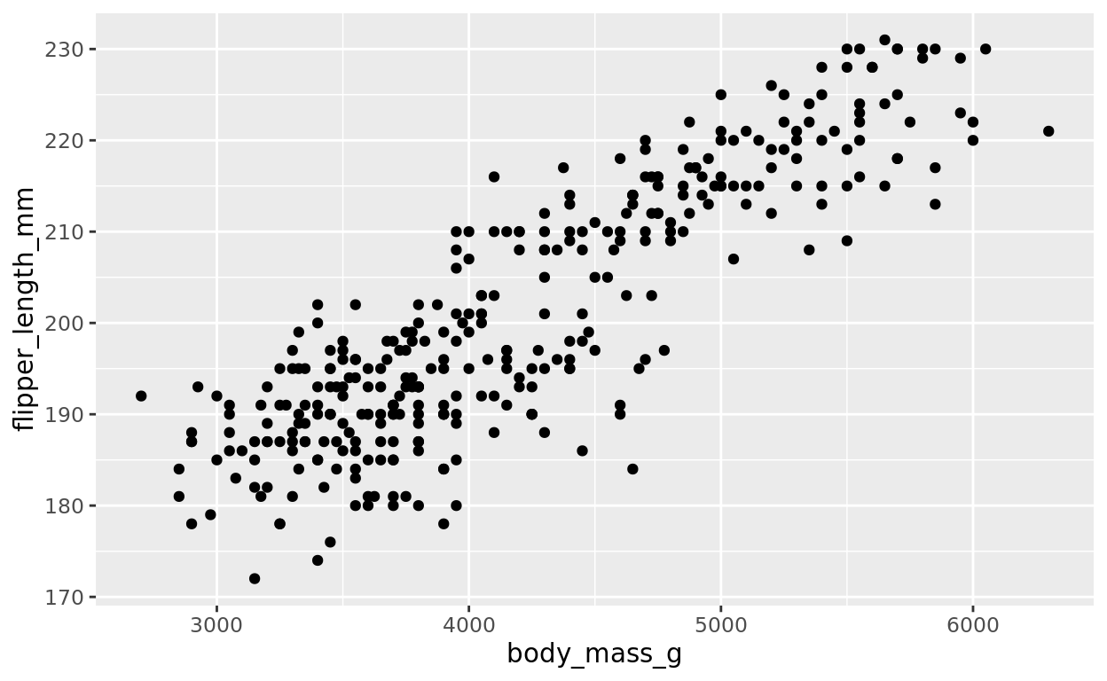

Formatting Reminders

As a reminder, we can add some formatting to make this look cleaner, or just make some stylistic choices!

• Titles/axis labels
• Change the point color
• plot themes
• Even transparency using alpha if our plot has a lot of overlapping dots, and we want to see the density of points more clearly.

ggplot(data = penguins, aes(x = body_mass_g, y = flipper_length_mm)) +
  geom_point(color = "purple", alpha = 0.3) +
  labs(title = "Flipper Length by Body Mass", y = "Flipper Length (mm)", x = "Body Mass (g)") +
  theme_bw()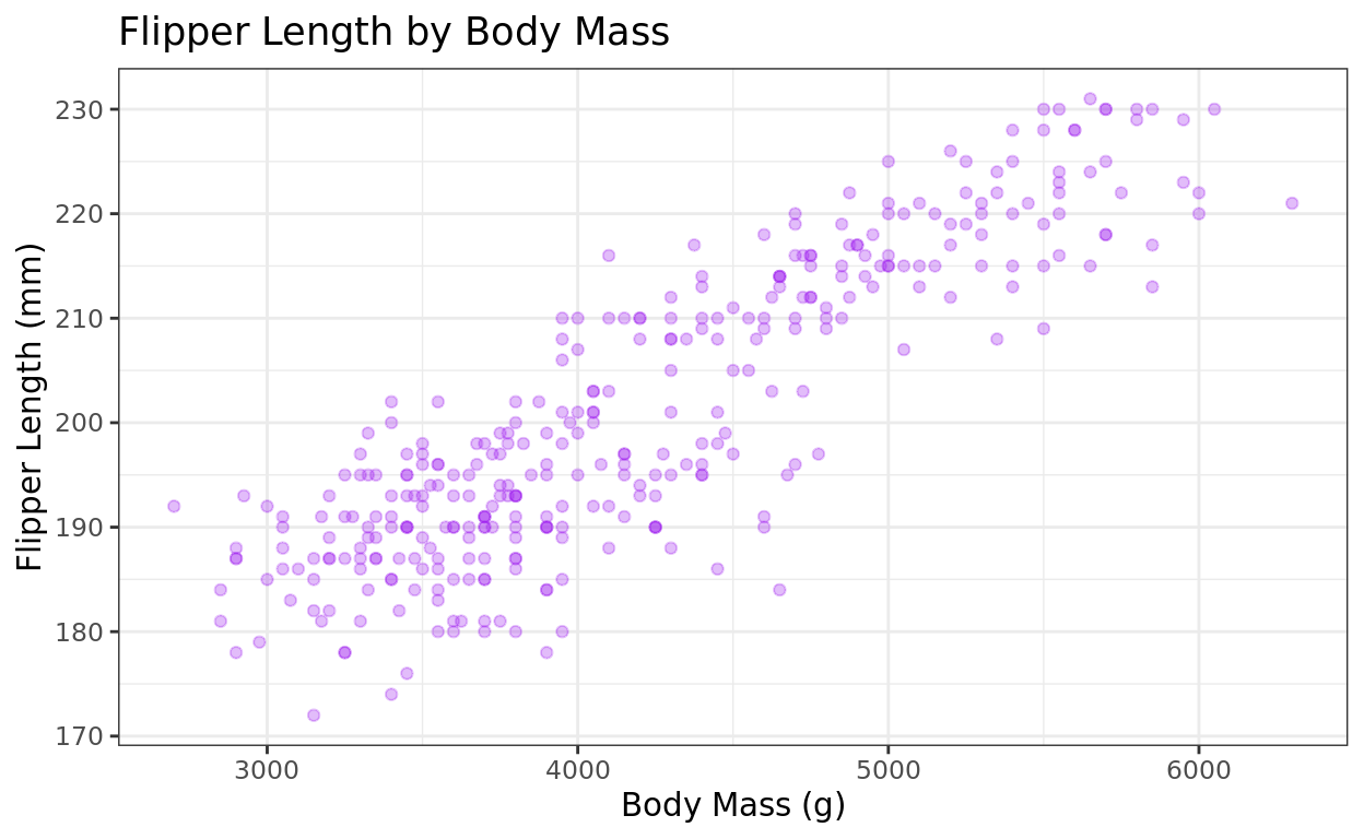

The transparency isn't really needed for this one--it's just here to demonstrate it. :)

Introducing geom_smooth

The geom_smooth function is one way to add a best fit line to our plot. The default line option it produces is the result of using the least-squares criterion to fit the line. We just need two arguments:

• method = "lm" (lm just stands for linear model, as opposed to some other type of model).
• formula = y~x (just means we aren't doing any predictor or response transformation.)

ggplot(data = penguins, aes(x = body_mass_g, y = flipper_length_mm)) +
  geom_point(color = "seagreen") +
  labs(title = "Flipper Length by Body Mass", y = "Flipper Length (mm)", x = "Body Mass (g)") +
  theme_bw() +
  geom_smooth(method = "lm", formula = y~x)

Don't need the formula line

I typically leave out the formula = y~x argument since that is the default relationship with geom_smooth. So feel free to just leave that out!

It gives you a message letting you know it's defaulting to a simple linear fit.

ggplot(data = penguins, aes(x = body_mass_g, y = flipper_length_mm)) +
  geom_point(color = "seagreen") +
  labs(title = "Flipper Length by Body Mass", y = "Flipper Length (mm)", x = "Body Mass (g)") +
  theme_bw() +
  geom_smooth(method = "lm")

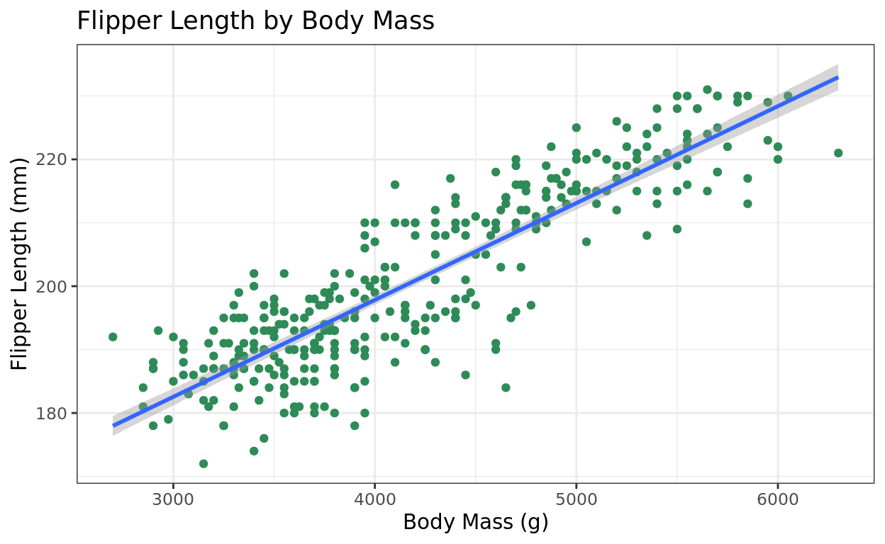
More geom_smooth options

Here are two other things you can customize:

• Femove the standard error shading: se = FALSE (usually what I do).
• Change the line color: color = "black" or whatever color you want.

ggplot(data = penguins, aes(x = body_mass_g, y = flipper_length_mm)) +
  geom_point(color = "seagreen") +
  labs(title = "Flipper Length by Body Mass", y = "Flipper Length (mm)", x = "Body Mass (g)") +
  theme_bw() +
  geom_smooth(method = "lm", se = FALSE, color = "gold3")

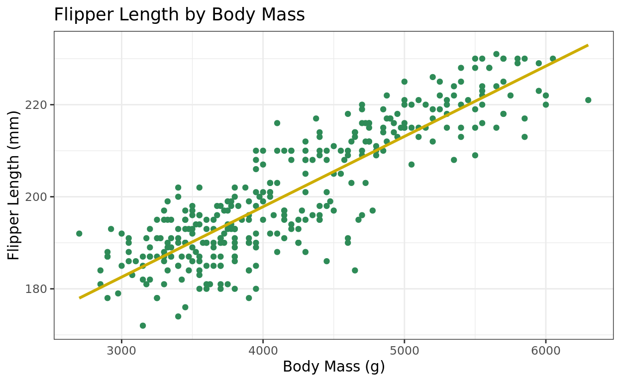
Try one?

Create a scatterplot using the diabetes dataset.

• Your x axis should be weightand your y axis as ratio.
• This data is dense, so add transparency with alpha (perhaps around 0.3)
• Add a best fit line, and turn off the standard error shading (keeping the color blue is fine)

Hint: Click "Hints" for a scaffold, and click through till you get to the full solution as needed!

ggplot(data = _______, aes(_______________)) +
  geom_point(_______) +
  _____________

ggplot(data = diabetes, aes(x = weight, y = ratio)) +
  geom_point(_______) +
  _____________

ggplot(data = diabetes, aes(x = weight, y = ratio)) +
  geom_point(alpha = 0.3) +
  geom_smooth()

ggplot(data = diabetes, aes(x = weight, y = ratio)) +
  geom_point(alpha = 0.3) +
  geom_smooth(method = "lm", se = FALSE)

Creating a Numeric Model

To get the coefficients of a best fit line, and a few other things, we can try creating a linear model with the lm function. This function takes:

• data: the name of the data frame containing variables you are modeling.
• formula, which will be in the form response ~ predictor

Adding our data

Let's create a simple linear model that predicts flipper length based on a penguin's body mass.

Running the code by itself will just offer the intercept and slope coefficient.

lm(data = penguins, formula = flipper_length_mm ~ body_mass_g)

What does that mean?

It means our best fit line predicting flipper length from body mass would be:

\(\hat{y} = 136.73 + 0.01528\)*(body_mass)

Model summary

Typically though, we'd like much more information. Go ahead and save your model to a descriptive name, and then run a summary of that model.

Notice that I'm also going to drop the formula argument name from here on, as R will recognize your input for that.

flip_model = lm(data = penguins, flipper_length_mm ~ body_mass_g)
summary(flip_model)

What does summary provide?

Here are three lines to focus on. Notice that the intercept and slope coefficients are in the "Estimate" column.

• The intercept coefficient = 136.7 (you can ignore the t-test results for the intercept)
• The slope coefficient = 0.01528, and in that same line, you'll also find
• the standard error for the slope = 0.0004668
• the test statistic for a t-test: t-value = 32.72
• the p-value = 2e-16 (at the end of the line, testing the null that the true slope = 0)
• The (multiple) \(r^2\) = 0.759; and adjusted \(r^2\) = 0.7583

We won't be using anything else in this output for now.

Interpeting the results

The t-test is testing against the null that the slope is 0. The p-value at the end of that slope line is extremely low. It's the lowest p-value that R will show in summary output (2e-16). This means we're VERY confident that there is at least some linear relationship here.

The adjusted r squared is 75.83%--knowing body mass helps us explains 75.83% of the variance in flipper length, after adjusting for correlation likely explained by random chance. That's quite a bit!

The F-test at bottom

The F-test on the bottom line is testing whether the model as a whole is performing better than the "null model" (just using the mean of the response variable as our best prediction).

• For a simple model, this will always match the p-value of our one coefficient's t-test.
• However, when models have two or more predictors, this will be different.

For our class, you can ignore this F-test result, as we'll focus on individual predictors, or just R squared to measure the full model's accuracy.

Quick Practice

How might we set up a linear model to predict the HDL/LDl cholesterol ratio based on weight in the diabetes dataset?

mod_ratio = __________________
______________

mod_ratio = lm(data = __________, _______ ~ _______)
summary(_________)

mod_ratio = lm(data = diabetes, ratio ~ _______)
summary(_________)

mod_ratio = lm(data = diabetes, ratio ~ weight)
summary(mod_ratio)

Interpretation quiz

Predicting

We can also use our model to fm make a model-based prediction for the response based on a plugged in predictor value.

predict

The predict function will take an inputted predictor value and then find the point on the best fit line as a best estimate for the response variable. It takes two arguments

• object: The model we created that we wish to use as the basis of our prediction
• newdata: a data frame of the predictor(s) we are plugging in.

For a simple model, newdata will be a data frame of only one column--our one predictor!

Try it out

Let's do that with our flip_model, where we will predict the flipper length of a penguin with a body mass of 4000g

flip_model = lm(data = penguins, flipper_length_mm ~ body_mass_g)

predict(object = flip_model, 
        newdata = data.frame(body_mass_g = 4000))

Multiple predictions

The newdata argument is also flexible enough to plug in multiple predictor values, allowing you to make multiple predictions at once.

flip_model = lm(data = penguins, flipper_length_mm ~ body_mass_g)

predict(object = flip_model, 
        newdata = data.frame(body_mass_g = c(4000, 4100, 4300)))